
Equality vs equivalence: computing isomorphism classes of C-sets
c-sets
attributed-c-sets
databases
For graphs and C-sets more generally, the most useful notion of equivalence differs from strict equality of the underlying data structures. Finding automorphism classes of C-sets addresses this problem; we explore how to compute automorphism classes and applications of them.
$$
$$
When is one thing equivalent to another? It turns out that answering this depends on a context, in some informal sense. Category theory offers a language by which this can be made precise, which has implications for a variety of technical challenges encountered in scientific computing.
Familiarity with C-sets in Catlab is helpful for understanding technical aspects later on in the post; however, readers new to AlgebraicJulia will benefit from reading about the motivation, the problem of graph equivalence, and the concluding thoughts.
Motivation
A common feature of both everyday conversation and esoteric arguments is the negotiation of whether or not two things can be called ‘the same’. These arguments are often fundamentally confused because it is difficult to be explicit about what we mean by ‘the same’. Consider these examples: - If Alice is in a political argument against Bob, she can charge Bob with hypocrisy for endorsing the same action as one he has previously condemned. Bob will then have to make a distinction (e.g. “that action is different in the context of miltary conflict!”), and the argument progresses from there. Likewise, Alice can defend herself by claiming her action is the same as that which Bob has previously endorsed. - Many debates are secretly about how to treat context: an artist taking a urinal or a Brillo soap box and presenting it as art will provoke controversy, given that one could argue that we have the same objects in our bathrooms (yet those are clearly not art). Likewise, one could argue about whether a novel written today that is word-for-word identical to Don Quixote could actually be a truly different work of art. And one could argue about whether a novel that is word-for-word identical to a meaningful work like Hamlet could actually be meaningless, in the context of a library that contains every possible book. - Does the Star Trek teleporter kill you? Is Theseus’ ship the same ship as before? It turns out questions of sameness and difference are also closely related to questions of identity: we often assert an identity of an object (e.g. a rock, a river, ourselves) across different moments in time, but we’re then forced to awkwardly say two things are “the same, but different”. This awkwardness and the ensuing confusion is the price paid in exchange for the brevity, clarity, and convenience we often gain by treating an equivalence relation as if it were an identity relation.
We also suffer when we are not explicit about what we mean by ‘the same’ while programming:
mutable struct Color
  name::String
  wavelength::Int
end

my_blue  = Color("blue", 470)
my_green = Color("green", 530)
my_blue == my_green # returns "false", as expected

your_blue = Color("blue", 470)
my_blue == your_blue # returns "false"!
The computer is not taking a philosophical stance, but rather it was asked to tell whether two things were equal without being told how to compute this. It guessed, using a default == method that is unsatisfactory for our use case. Given that we actually would like to say these two blues are the same, we can manually define an equality test method to improve things:
# Ask yourself: is this reasonable?
Base.:(==)(x::Color, y::Color) = x.wavelength == y.wavelength

my_blue == your_blue # now returns "true" as desired

aqua = Color("aqua", 500)
cyan = Color("cyan", 500)
cyan == aqua # returns "true", but should it?

grue = Color("grue", if (CURRENT_YEAR < 2100) 530 else 470 end)
grue == my_green # returns "true", but should it?
So even in technical situations, whether or not two entities are equal can be nebulous. The dilemma is this: providing explicit == algorithms is often undesirable because it feels tedious and mechanical, like something that should be automated; however, there is no unopinionated way to pick a default looking at the data alone. A solution to this dilemma is make it convenient to work with data alongside their contexts, which provide enough information for sameness to be determined algorithmically. Namely, when an entity is regarded as the object of a category, we obtain a formal notion of equivalence that, in many scenarios, captures what we intend by the == operator.1
In Catlab.jl, we use a data structure called an attributed C-set (or ACSet) to manipulate data that is situated within a category. This generalizes a broad class of data structures, including many generalizations of graphs (e.g. directed, symmetric, reflexive), tabular data (e.g. data frames), and combinations of the two (e.g. weighted graphs, relational databases). Here, we’ll discuss the benefits of working with isomorphism classes of ACSets, i.e. ACSets up to isomorphism. A working implementation of the code presented below can be found at CSetAutomorphisms.jl.
Equality vs equivalence: graphs
A key insight of modern mathematics is that equality is often more strict of a notion than what we want in practice. When reasoning about complex mathematical structures we need to shift our perspective to interchangeable in this context. Let’s consider directed graphs as an example:
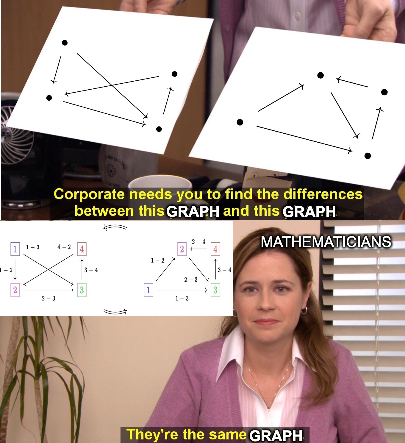
Of course, the pictures of the graphs are different, but it’s crucial that graphs are different from images of graphs. Mathematicians regard the two graphs above as equal in the context of graph theory because the graphs cannot be distinguished in the language of graph theory. However, a computer must go beyond this language by labeling vertices and edges in order to efficiently represent a graph:
The three edges of this graph can be represented by two vectors of length three: src=[1,1,2], tgt=[2,3,3],src=[2,1,1], tgt=[3,3,2].

And should it be the same graph if we keep the arrow order but identify the vertices differently? We want the answers to these questions to be yes.
However, this is harder than it seems at first; the computer has direct access only to the underlying vector representations, which are not strictly equal in the above cases. In general, it is a tough computational problem (the graph isomorphism problem) to answer whether two graphs are equal in this richer, more meaningful sense because it involves searching over all possible reorderings of the labels.
The problem is even worse if we are frequently searching whether a graph is contained in some database of 1,000,000 graphs: each time we query, we’d have to solve the graph isomorphism problem up to 1,000,000 times! A solution to this problem is to find a canonical labeling, i.e. a specific labeling (out of all isomorphic labelings of a given graph) which is designated to be the representative. Given a method to compute this, we turn a hard problem (are two graphs isomorphic?) into an easy one (are the graphs’ canonical labelings strictly equal?). This labeling can then be used as a fingerprint to quickly check if the graph of interest is in the database: at worst, 1,000,000 string equality tests. The only challenge is to compute the canonical labeling of just our one graph of interest.
Working Example: ACSet for chemical reactions
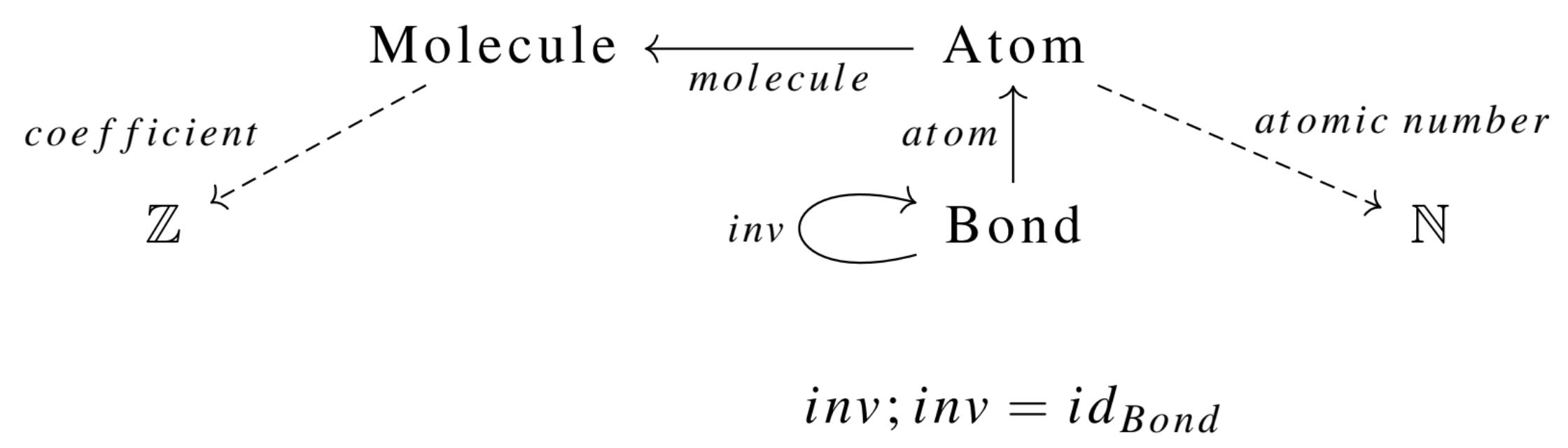
Much time and effort has been spent crafting efficient algorithms to solve the canonical graph labeling problem, with the most popular software being Nauty (McKay and Piperno 2014), written in C. Most high-level languages that solve this problem do so by constructing input that is passed to the original Nauty program. However, what should be done if we care about things that aren’t graphs? For example, an ACSet representing chemical reactions, specified by the following schema:2
This is the declaration in Catlab.jl (full code in CSetAutomorphisms.jl):
using Catlab, Catlab.Theories, Catlab.CategoricalAlgebra

@present SchRxn(FreeSchema) begin
  (Molecule, Atom, Bond)::Ob
  inv::Hom(Bond,Bond)
  atom::Hom(Bond, Atom)
  mol::Hom(Atom, Molecule)

  (Float, Num)::AttrType
  atomic_number::Attr(Atom, Num)
  coefficient::Attr(Molecule, Float)

  compose(inv, inv) == id(Bond)
end

@ACSet_type RxnGeneric(SchRxn)
Rxn = RxnGeneric{Float64, Int}
This ACSet schema defines a category of chemical reactions, and viewing a mathematical entity as the object of a category gives us a natural context for determining when things are equivalent. This particular category captures many domain-specific features of the data that are not captured by representing the reaction as a simple struct of various tuples and lists of data: - Neither the ordering in which atoms are labeled, the ordering of atoms within bonds, nor the ordering of bonds themselves is relevant to the identity of a molecule. - The ordering in which the reactant molecules or product molecules are listed is not relevant to the identity of the reaction: we want 2 H_2O \rightarrow 2 H_2 + O_2 to be the same as 2 H_2O \rightarrow O_2 + 2 H_2 - The atomic numbers are relevant to molecule identity: CO_2 is not H_2O because atomic number is an attribute rather than a piece of combinatorial data. Likewise for the coefficients on the reactants and products. - Stoichiometric coefficients distinguish the reactants (negative coefficients) from the products (positive coefficients), which is particularly important if we wish to characterize reactions with properties such as exothermicity.
In Catlab, we can declare both 2 H_2O \rightarrow 2 H_2 + O_2 and 2 H_2O \rightarrow O_2 + 2 H_2 with the following code:
H2 = @ACSet Rxn begin
  Molecule = 1
  coefficient = [2.0]
  Atom = 2
  atomic_number = [1, 1]
  mol  = [1, 1]
  Bond = 2
  atom = [1, 2]
  inv  = [2, 1]
end

O2 = deepcopy(H2)
set_subpart!(O2, :coefficient, [1.0])
set_subpart!(O2, :atomic_number, [8,8])

H2O = @ACSet Rxn begin
  Molecule = 1
  coefficient = [-2.0]
  Atom = 3
  atomic_number = [1, 1, 8]
  mol  = [1, 1, 1]
  Bond = 4
  atom = [1, 3, 2, 3]
  inv  = [2, 1, 4, 3]
end

rxn₁, rxn₂ = Rxn(), Rxn()
[copy_parts!(rxn₁, x) for x in [H2O, O2, H2]]
[copy_parts!(rxn₂, x) for x in [H2O, H2, O2]]

println(rxn₁ == rxn₂) # false
println(is_isomorphic(rxn₁, rxn₂)) # true
Catlab’s is_isomorphic function offers a solution to the graph isomorphism problem that works generically for any ACSet. However, returning to the paradigm use case for canonical isomorphisms, a scientist requires a canonical labeling in order to efficiently query a large database of reactions and see if a particular reaction is inside. This problem is addressed in CSetAutomorphisms.jl, where we generalize the Nauty algorithm beyond graphs to ACSets. The brief summary below, as well as the implementation, are based on this lucid expository paper (Hartke and Radcliffe 2009) on the Nauty algorithm. Formal statements can be found there for aspects of the algorithm that are shown here only by example.
Generalized Nauty Algorithm
Considering data up to isomorphism is easy for a mathematician (it’s just forgetting information!) but difficult for a computer, requiring a complicated algorithm. This algorithm has three main ingredients: color saturation, search tree exploration, and automorphism pruning. These will be briefly explained and shown to require only minor modifications to generalize to arbitrary ACSets, with our earlier ACSet rxn₁ as a running example. We ignore attributes, which are discussed later, meaning that we should now think of rxn₁ not as ⬤-⬤-⬤ -> ⬤-⬤ + ⬤-⬤.
Overview
While one can think of vertex labels 1,2,3,4 as natural numbers, it can also be helpful to think of the labels as colors: 🔵, 🟢, 🟠, 🔴 (ordering could come from alphabetizing). This shift is helpful when thinking about labelings as partitions of a set. We can refine a partition by making it more specialized (splitting up colors, never merging colors).
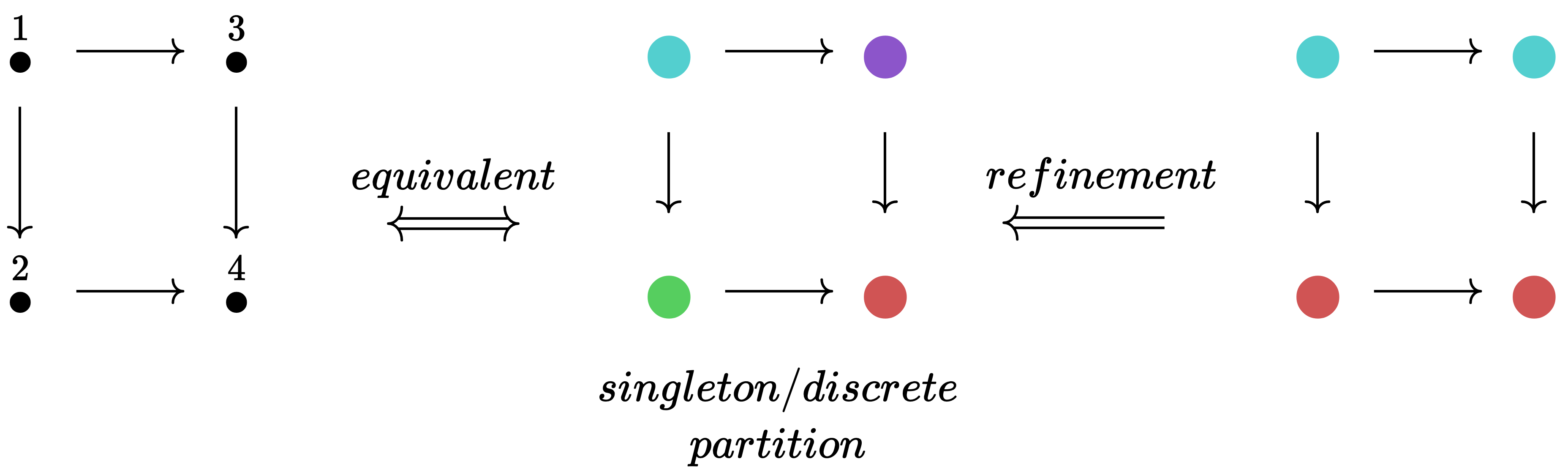
This refinement process can go no further when we reach a singleton partitioning (or discrete partitioning), where each element has its own color. Because such a coloring can be translated back into distinct natural numbers, it can be thought of as a permutation. While a permutation is an isomorphism of an object with itself in the category Set, we use the word automorphism to refer to the general case of an isomorphism from an object of some category to itself. When we are in an C-set category, the required data of an automorphism is a set permutation for each object in the indexing category.
Once we find all refinements that are automorphisms, we have identified the isomorphism class of our input C-set and can select a canonical element by taking the lexicographic minimum.3
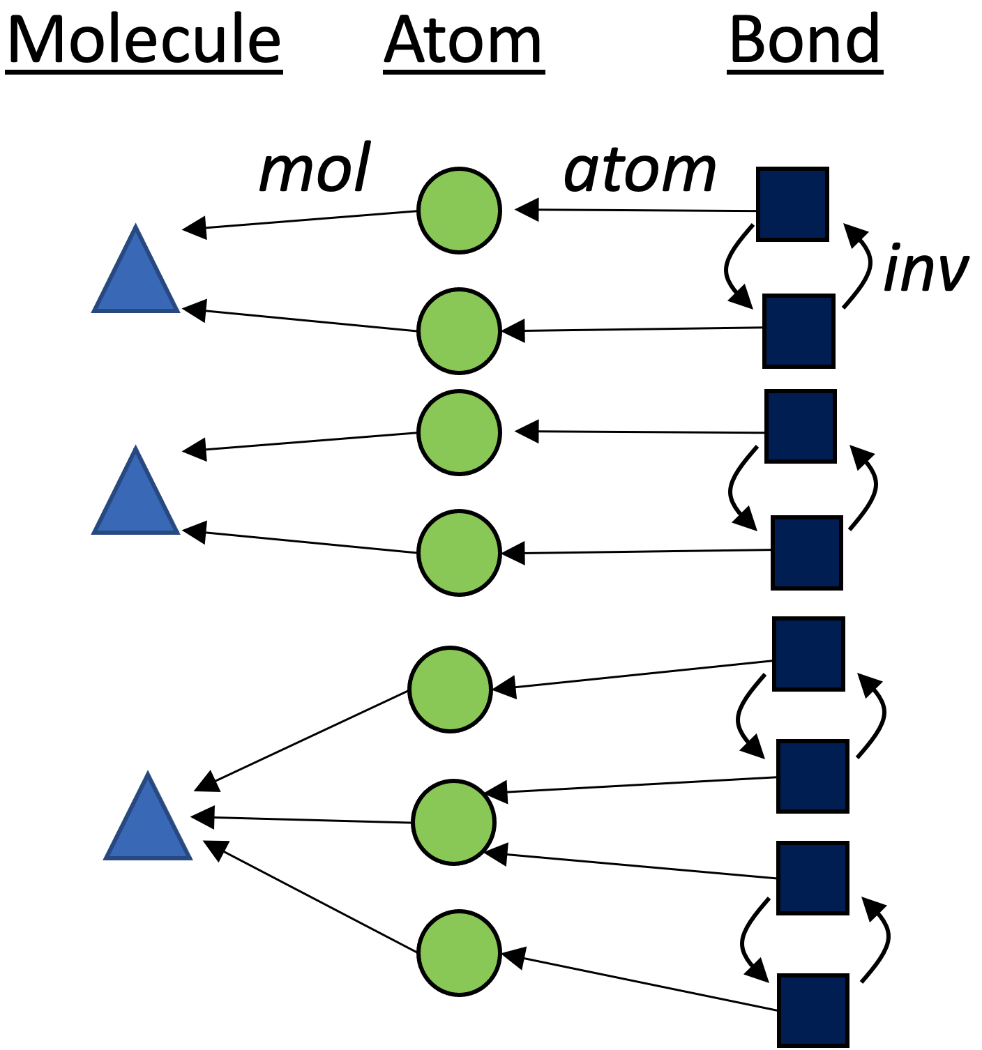
Below is a graphical depiction of rxn₁.4 Our starting point has no information as to what the automorphisms are, which is reflected by the fact that all three partitions are as unrefined as possible.
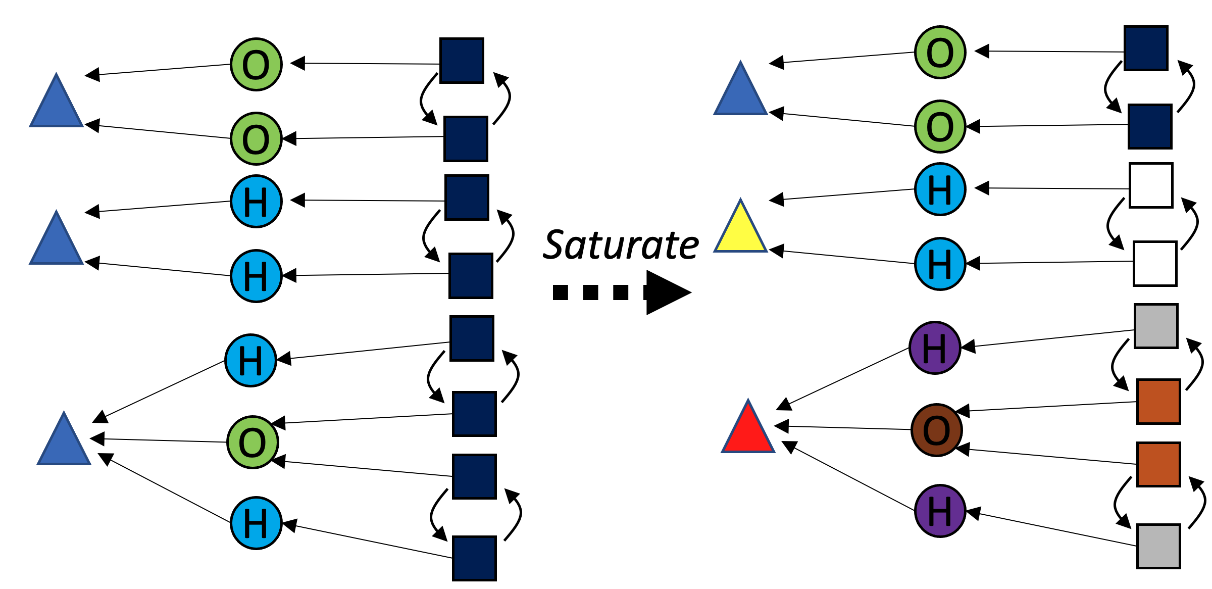
Color saturation
Color saturation is a method of refining colorings of a graph without ruling out automorphisms. For graphs, we first collect data on the “local environment” of each vertex (how many of each color is adjacent). Because we can canonically order local environment data, we can canonically recolor the vertices by their local environment. This procedure can be repeated until convergence. Color saturation brings us closer towards our goal of identifying all automorphisms, but it does not completely solve our problem (sometimes it cannot make progress at all, e.g. starting with a complete graph).
With C-sets, there is an analogy to the “local environment” of graphs, demonstrated for the green {\rm Bond} box with the asterisk in the following figure:
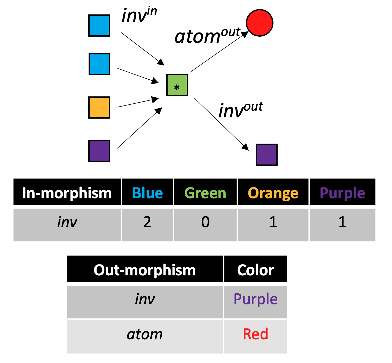
Each iteration of color saturation is a refinement. The refinement of rxn₁ has three steps, as shown below.
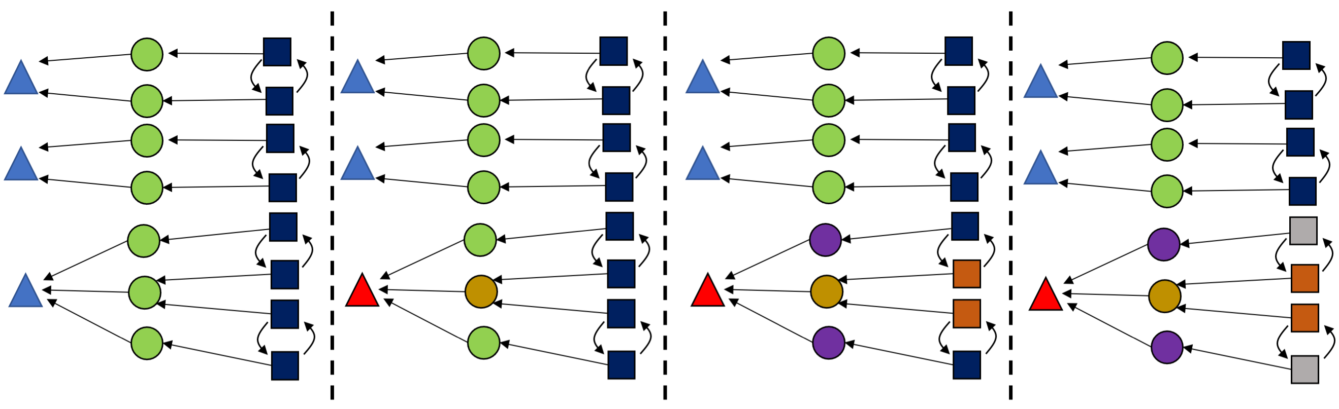
This is relatively cheap to compute and can greatly reduce the search space, so we color saturate not only at the beginning but also throughout the algorithm, each time we learn new information.
Search tree exploration
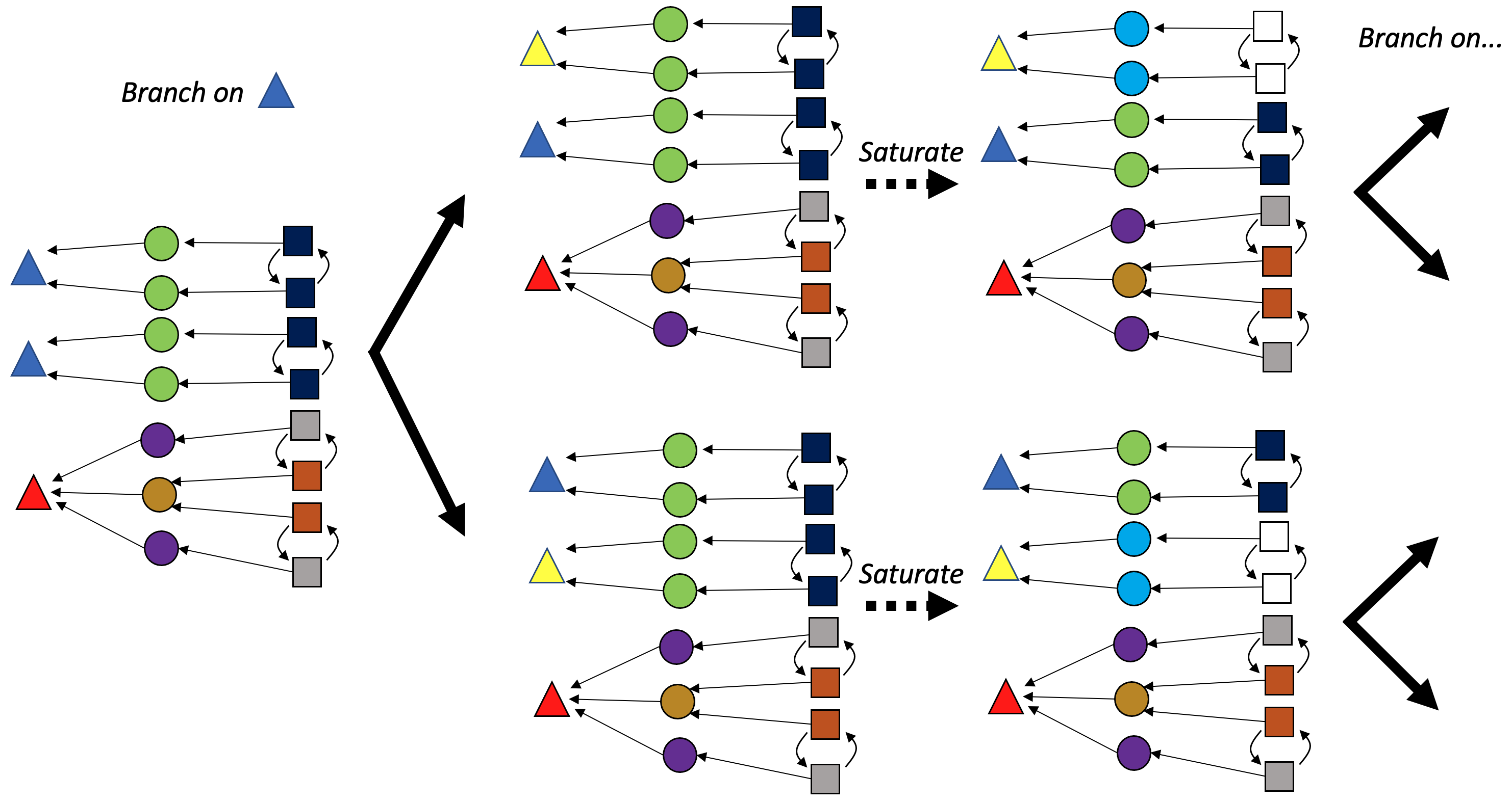
Suppose that color saturation has refined our partition as far as it can. How do we identify which subset of the singleton refinements are valid automorphisms? In theory, we must try all \displaystyle \prod_{c\in Colors} |c|! combinations of each individual color’s permutations. These are all possible ways of completely breaking each symmetry. To avoid this combinatorial explosion, the search tree approach breaks one symmetry at a time (branching on the possible ways to do this) and runs color saturation immediately, which allows us to take advantage of the graph’s connectivity structure to do most of the refinement heavy lifting.
More precisely, our tree has graph colorings as nodes and edges to children nodes are “artificial distinctions”: all possible refinements that break the symmetry of a particular color (which can be chosen canonically) that add one new color.5 Finding all of the leaves of this tree is our goal: these are all possible singleton colorings that are valid automorphisms.
These ideas straightforwardly generalize to C-sets, where we maintain colorings for each component, rather than just for vertices. We still break symmetry for just one color (of a single component) when branching in the search tree.
Automorphism pruning
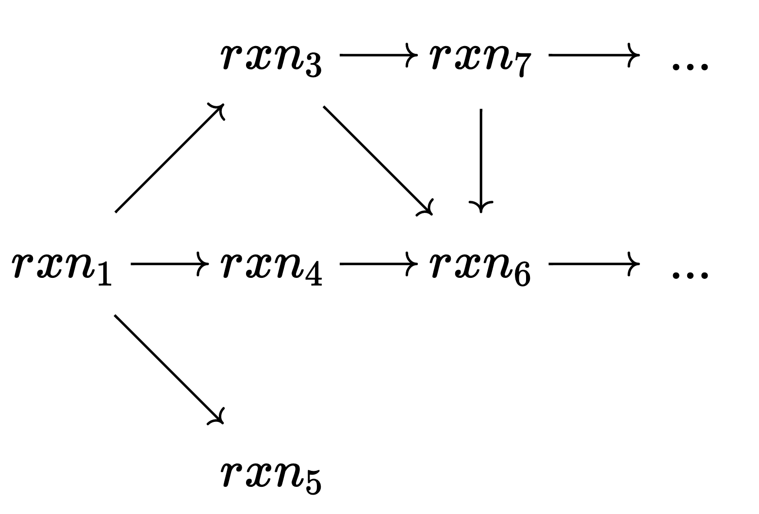
The search tree can be extremely large, even when applying color saturation whenever possible. Thankfully, because we explore the search tree depth-first, we can use the leaves we’ve seen already to sometimes determine that there is no new information below a certain node, and thus its children do not need to be explored.
Referring to the previous figure for intuition: our initial split effectively differentiated the two diatomic molecules. In each branch remains much work remaining to be done in order to reach a singleton coloring; however, we have an intuition that there will be some redundant work if we consider these two branches as fully independent (after all, we know we’re making a distinction between two molecules that are truly interchangable). This intuition can be formalized by the following rule:
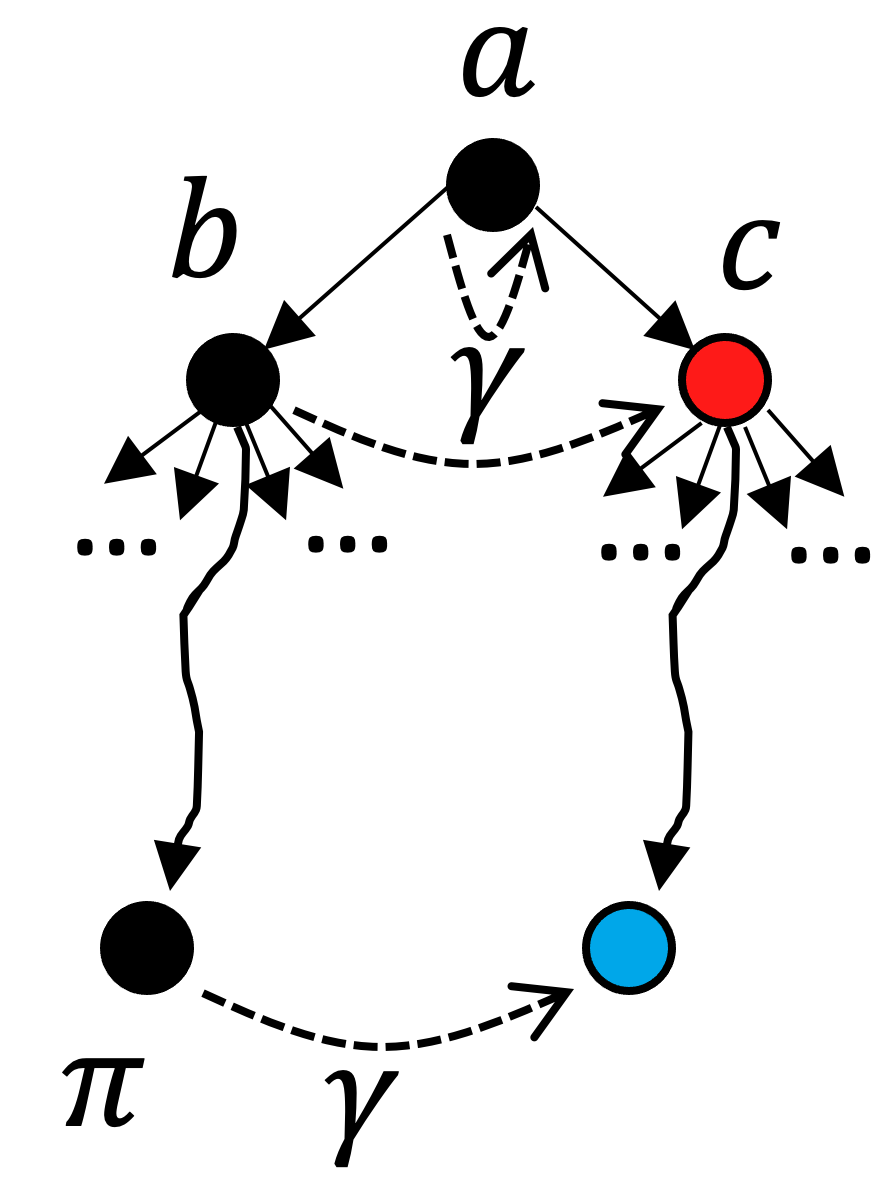
In this image, a corresponds to our initial color saturation result, and b and c are the two results for our initial branching. In this scenario, we have fully explored the search tree beneath b. The black nodes have already been explored and we’re contemplating branching on node c. So far we have discovered automorphisms (leaf nodes) \pi and \gamma. Despite the fact that there is an unexplored leaf node under c (in blue), we can actually prune c from the search tree if it turns out that \gamma preserves a (the nearest ancestor of b and c) and maps b into c. This is the formal specification for our intuition that the two diatomic molecules being the same means we oughtn’t have to explore both branches: the subtree under b is isomorphic to the subtree under c if this property holds. Note that this reasoning is purely categorical - because it is purely defined in terms of morphisms, it works equally well in ACSet categories as it works in Grph.
Extending from C-Sets to ACSets
Attributes that come with an inherent ordering make this problem easier rather than harder, as the non-combinatorial data they provide can be used to distinguish elements during color saturation. All typical attributes have this property: Int, Float, String. In the color saturation example above, atomic\_number would immediately allow us to distinguish the O_2 molecule from the H_2 molecule.
In the case of an attribute without an ordering to use, we can create a pseudo object with a number of elements equal to the number of distinct values found in the ACSet, e.g. if the datatype of {\rm Coefficient} were hypothetically not inherently ordered, we could create a {\rm Coefficient} object with three elements inside and then then run the algorithm as normal. This is less preferable because it requires computational work to come up with a canonical labeling of the pseudo C-set object.
Outlook
Viewing a particular piece of data in the context of a category provides us enough context to resolve tricky issues of determining what is effectively the same as what. Due to the generality of the applied category theory perspective, we automatically bypass the tedious process of defining __eq__ and __hash__ methods for each new data structure we invent.
This is an exciting development because it enables hashing C-sets, a crucial operation for many data structures (e.g. Dict{ACSet, String}) and algorithms. In particular, for dynamic programming algorithms, one can now incorporate C-sets into a state space and quickly check whether a state has already been seen. For example, suppose we have experimental data for H_2, O_2, and H_2O and hypothesize that rxn₁ is right model for this. An iterative algorithm could evaluate the proposed reaction against the data and propose modifications to rxn₁ that would improve the quality of fit. This yields a search space of {\rm Rxn} objects with intersecting paths. In such a scenario, we can greatly reduce computations that need to be done by checking if a new {\rm Rxn} is actually new when considered up to isomorphism.
Furthermore, the notion of a ‘random’ C-set instance crucially depends on which notion of equality we consider: picking a random instance of the C-set data structure (in contrast to picking a random C-set isomorphism class) will heavily overrepresent isomorphism classes with many elements. Using the isomorphism class notion of randomness is important in statistical mechanics applications and more closely matches what one means when discussing a random directed graph or a random Petri net.
As a final thought, the difficulty of implementing new algorithms often leads one to reduce one’s problem into the form of another problem which has a ready-made algorithm. Although the ACSet of reactions is a richer, more complex structure than a graph, it is possible to encode it as a graph such that existing Nauty code can be used to perform the computation. Call this “bringing the data to the algorithm”. This process takes time, can create large constant factors (by encoding rich structures in a simpler language), and prevents us from taking advantage of higher-order structure lost in the translation. We avoid these pitfalls by working at a higher level of abstraction: implementing an algorithm once for C-sets and letting Julia generate specialized code for each concrete data structure that is a C-set instance. In our experience, most graph algorithms (including complicated ones, such as Nauty) straightforwardly generalize to ACSets, making us optimistic about a future where we “bring the algorithm to the data”.
References
Hartke, Stephen G., and A. J. Radcliffe. 2009. “McKay’s Canonical Graph Labeling Algorithm.” American Mathematical Society. https://doi.org/10.1090/conm/479/09345.
McKay, Brendan D., and Adolfo Piperno. 2014. “Practical Graph Isomorphism, II.” Journal of Symbolic Computation 60 (January): 94–112. https://doi.org/10.1016/j.jsc.2013.09.003.
Footnotes
We recommend referring to this context-sensitive equality as ‘equivalence’, in contrast to ‘literal’ or ‘strict’ equality. As Eugenia Cheng advocates, “All equations are lies…or useless.”↩︎
The relation between bonds and atoms is taken from half-edge graphs, which encode symmetric relationships and also allow for the representation of ‘dangling bonds’.↩︎
For example, the graph with two vertices and an arrow going between them has two elements in the automorphism class: G_n:=(src=[1],\ tgt=[2]) and G_m:=(src=[2], tgt=[1]). Because the underlying data of a C-set is essentially of type
Dict{String, Vector{Int}}, we require a method to tell whether two elements of this type are less than, greater, or equal to each other. One way to do this is to order the vectors (in this case, let’s use alphabetization to order the set \{src,\ tgt\}) in order to get two elements of typeVector{Vector{Int}}which we can compare to see that G_n \lt G_m.↩︎Although the elements of {\rm Molecule} (triangles), {\rm Atom} (circles), and {\rm Bond} (squares) live in different sets, we visualize them all in one graph via the category of elements construction.↩︎
For example, with 🔴🟡🟡🔴🟡🔴🔴, we branch on 🟡 and obtain three child nodes:
🔴🟢🟡🔴🟡🔴🔴, 🔴🟡🟢🔴🟡🔴🔴, and 🔴🟡🟡🔴🟢🔴🔴. ↩︎