Acsets with variables
$$
$$
A central data structure in AlgebraicJulia is the acset, short for attributed \mathsf{C}-set. For background on acsets, see this blog post, or the original paper (Patterson, Lynch, and Fairbanks 2021). \mathsf{C}-sets store combinatorial data, which consists of sets of indistinguishable objects (such as the vertices of a graph) related by functions. Acsets extend this to include non-combinatorial data, which consists of things with intrinsic meaning such as integers, strings, and so on.
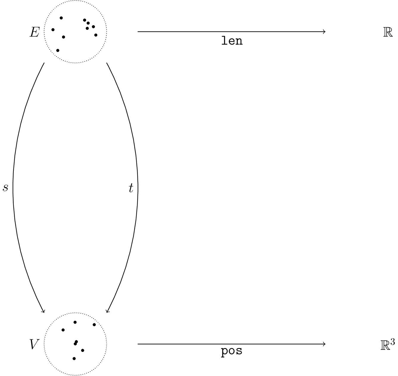
To recall notation, in order to give a category of acsets we first give a schema, a profunctor {S:S_0\nrightarrow S_1}. Then an acset is a copresheaf F:|S|\to \mathsf{Set} on the collage of S with a fixed restriction K to S_1 giving the attribute types, for which reason we’ll call K the “typing map.” The morphisms of acsets thus fix everything in K exactly. For example, a morphism A \rightarrow B between \mathbb{R}-weighted graphs can in principle send any vertex in A to any vertex in B, but we are required to send an edge of weight 2.2 in A to an edge of weight 2.2 in B.
But for many purposes this is too restrictive. This post is about a generalization of attribute types that allows us to have special attribute values, called variables, which can freely map to concrete values. A major motivation for developing this generalization is to support rule-based rewriting for acsets. We’re implementing these ideas today in our library Algebraic Rewriting.
As an example scenario, suppose we are trying to program a robot to assemble objects of various shapes from raw materials. Our first job in modeling this scenario is to pick a schema to represent the state of the world, as perceived by the robot. We’ll use a schema for mechanical linkages, which we’ll model as an attributed symmetric graph, where edges represent links using a length attribute, and vertices represent positions using a coordinate attribute.1

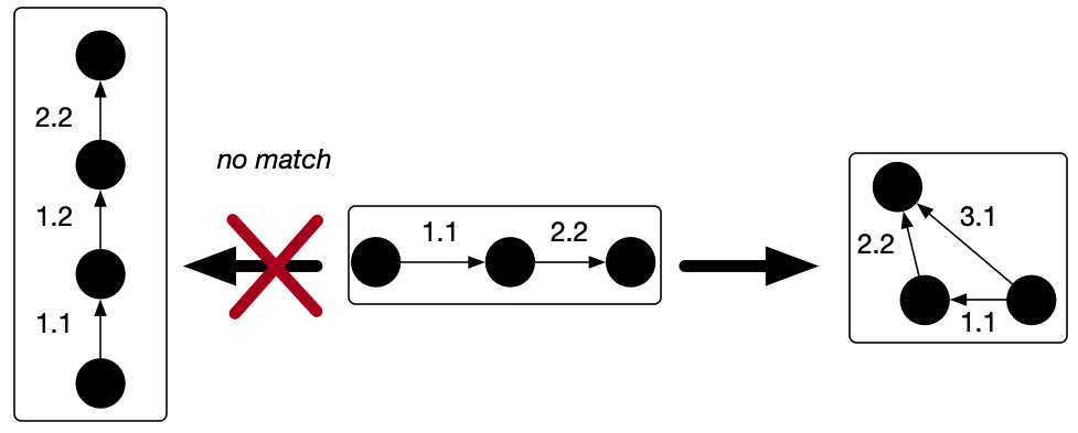
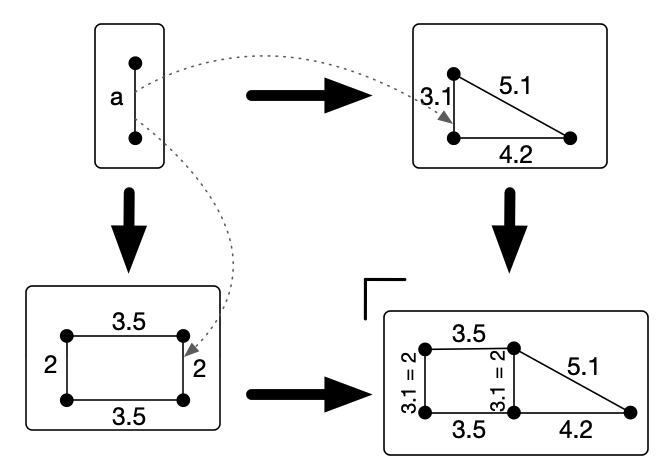
As an illustrative rewriting rule, let’s suppose that, whenever our robot sees a rectangular figure, it is allowed to tear the top off and fold the remaining open shape into an isosceles triangle. We can draw this fact as a rewriting rule; however, a well-formed acset requires us to put concrete attribute values for all the lengths and positions:
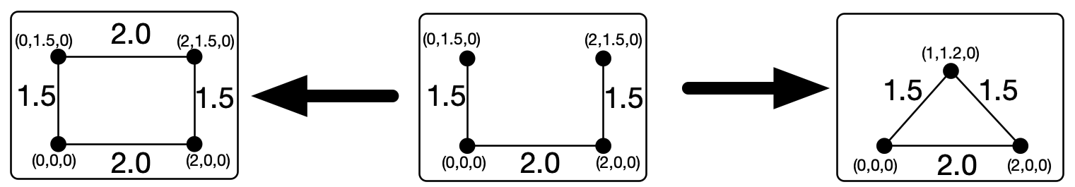
Having been forced to pick particular values, we are then unable to apply the rule to any rectangles of different dimensions (or located at different coordinates). The notion of a variable which can map into an arbitrary concrete value will allow us to write the rule we intended to write.
What’s a varacset?
Varacsets, short for “variable-equipped acsets”, allow for a supply of distinguishable variables from attribute types, which can be mapped to constants under acset morphisms. This should leave our rewrite rule looking something like this (with position variables omitted for brevity):
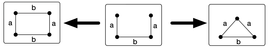
By allowing a set of distinguishable variables, which can explicitly be equal or not equal to each other, rather than merely extending the attribute type \mathbb{R} to include a wildcard element, {\mathbb{R}+\{*\}}, we can model a parallelogram with the leftmost acset, rather than an arbitrary quadrilateral.
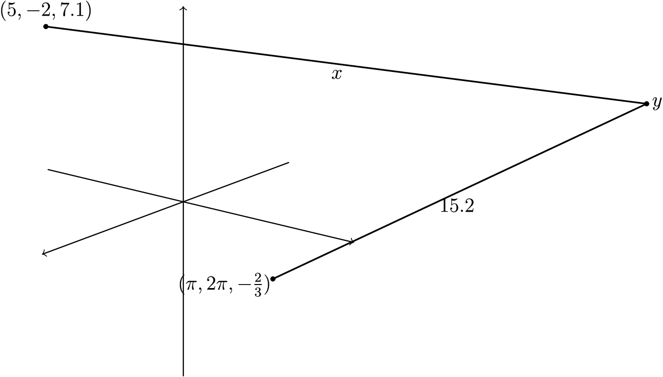
Although we can visualize these varacsets as undirected graphs, varacsets on any schema can be viewed as a set of tables in its database representation:
| V | \texttt{pos} |
|---|---|
| 1 | (5,-2,7.1) |
| 2 | \mathbf{AttrVar}(1) |
| 3 | (\pi,2\pi,-2/3) |
| E | x | t | \sigma | \texttt{len} |
|---|---|---|---|---|
| 1 | 1 | 2 | 2 | \mathbf{AttrVar}(1) |
| 2 | 2 | 1 | 1 | \mathbf{AttrVar}(1) |
| 3 | 2 | 3 | 4 | 15.2 |
| 4 | 3 | 2 | 3 | 15.2 |
What’s the category of varacsets?
Although the objects of acsets are the same as relational databases, they are much more powerful because we understand them as a category and can perform categorical constructions. Thus it’s important to understand how varacsets are a category such that we can find homomorphisms and compute (co)limits.
Defining the category
Let’s figure out what the category of varacsets looks like more precisely. Given a schema S_0\nrightarrow S_1, we start with a typing map K:S_1\to \mathsf{Set} which gives the values of each attribute type. Our full varacset should augment this data with combinatorial data over S_0 and a supply of variables over S_1, plus the actual attribute functions. Furthermore, we want to end up in a category where the morphisms fix the constants of each attribute type but move variables freely. This defines a category well enough, but its nature isn’t very clear.
Why a different approach from acsets is needed
Acsets as a slice category of \mathsf{C}-\mathsf{Set}
In the original acsets paper, the authors proved that the category of acsets with attribute types determined by K:S_1\to \mathsf{Set} is equivalent to the slice category of \mathsf{Set}^{S_0} over a certain functor K' closely related to K. This characterization is very helpful in seeing that the category of acsets with fixed typing is friendly (indeed, a topos), but it’s not computationally usable, because the functor K' (a certain right Kan extension) is generally something badly infinite. But the most interesting computations we can do in AlgebraicJulia, such as acset homomorphism search, depend on looking at acsets whose values over S_0 are finite sets. In any case, this trick can’t be readily imported to our situation, because the analog of K' would depend on the variables present in each particular acset and not only on the schema.
Flipping the slice
While the collaginess of |S| sure makes us want to think of F being over K in some sense, this is largely an illusion. What’s much more straightforward to formalize is a view of F as under a relative of K: namely, the functor K_! which adds empty values over S_0 to extend K to all of |S|.
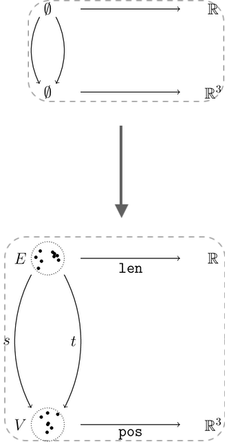
Indeed, the coslice category K_!/ \mathsf{Set}^{|S|} is awfully close to the category of acsets. Specifically, if you restrict to the full subcategory of the coslice spanned by maps from K_! which are invertible over S_1, then this is equivalent to the category of acsets as defined above. Indeed, maps in K_!/ \mathsf{Set}^{|S|} have to leave the image of K, i.e. our attribute values, put, but are just any old natural transformations on the rest of the functor, i.e. our combinatorial data.
For varacsets, we don’t want a coslice object K_!\to F which is iso over S_1, though. Instead, since we want to be able to add variables to our attribute types, we’d better relax at least to a mono. And that’s really all you have to do! The key observation is that variables in the attribute types behave precisely like combinatorial data: we can permute them around however we want without changing the meaning of an acset. This is basically the category we have implemented in AlgebraicJulia today: the full subcategory of K_!\downarrow \mathsf{Set}^{|S|} on monomorphisms.
Final definition
The nicest definition of a category of varacsets with attribute types given by K:S_1\to\mathsf{Set}, though, is simply the entire coslice category K_!\downarrow \mathsf{Set}^{|S|}, without the monicity restriction. One can imagine applications of the case where the coslice morphism is non-monic; for instance, such a varacset on the weighted graph schema would allow us to mix ordinary weighted graphs, with edges weighted in \mathbb R, with “angled graphs”, with edges weighted in the circle, \mathbb R/2\pi. In this case, the component of the coslice structure map at the weights object would be the canonical projection from the line to the circle.
Is this good? Maybe! In any case, the full coslice category has much better mathematical properties than the mono-coslice category. We will show in the next section precautions we can take if we wish to maintain the monicity restriction in practice.
Wandering variables
We can also define wandering variables as elements over some A\in S_1 that are not in the image of any attribute function. Varacsets with no wandering variables have some good properties; for example, only if X has no wandering variables can we enumerate morphisms {\alpha: X \rightarrow Y}. (In database theory lingo, we could say that such an acset has all its variables in the active domain.)
To illustrate, when each weight variable in a weighted graph has an associated edge, the regular acset search algorithm (which finds all compatible assignments of edges and vertices) will homomorphism determine where the edge weights must be sent via the naturality condition associated with the weight attribute (\alpha_E\cdot Y_{weight} = X_{weight}\cdot \alpha_{\texttt{Weight}}). However, a wandering variable’s image is not determined by this constraint, and in principle it could map to any weight variable in Y as well as any concrete value in \mathbb{R}. This means there would be an infinite number of morphisms X \rightarrow Y. We’ll see further below that the category of acsets without any wandering variables is better-behaved than you might expect.
Computing colimits
The coslice K_!\downarrow \mathsf{Set}^{|S|} is complete and cocomplete, and more: it’s not a topos anymore, but it is the category of models of a multi-sorted algebraic theory, which is pretty good.2 The monos-only category won’t even be cocomplete, since for instance pushouts will screw up mono-ness. In contrast, K_!\downarrow \mathsf{Set}^{|S|} has colimits computed mostly as in \mathsf{Set}^{|S|}, that is, levelwise; you just have to replace coproducts with pushouts under K_!, and similarly for other colimits over non-connected diagrams.
In terms of varacsets, passing to the full coslice category allows us to consider something like the pushout of a span whose legs send a variable-weight edge to edges of two different constant weights.
In the pushout, we just won’t be able to distinguish those two weights from each other anymore. If they don’t need to be distinguished, then this is great! That said, we generally only expect to be computing colimits that don’t require gluing together terms of the type of constants in an attribute, and so far we do not support any means of representing the resulting infinite sets with some elements marked as equivalent. So, with the caveat that we throw a runtime error in case concrete attribute values get identified, the colimits coming from K_!\downarrow \mathsf{Set}^{|S|} are doing exactly what we want.
Computing limits
Varacsets are an unusual category in which limits are trickier than colimits. To be sure, the limits in a coslice of \mathsf{Set}^{|S|} are computed exactly as in \mathsf{Set}^{|S|}, that is, levelwise. However, these limits have some issues, semantically. For instance, suppose you take the product of, say, two weighted graphs, with weights valued in \mathbb R. Then the product in K\downarrow \mathsf{Set}^{|S|} is going to have the weights valued in \mathbb R\times \mathbb R and \mathbb{R}^3\times \mathbb{R}^3, which is a whole different kind of situation!
While this is categorically-correct behavior, it’s not what we want in practice. Instead, we’d really like to make a construction that’s at least product-like that does not change the datatypes of attributes. It’s actually harder than you might guess to find a category in which to do this. The mono-coslice category we discussed earlier has the same products as the full coslice, and the need to allow for variables stops us thinking about the iso-coslice.
For further comparison, in the original slice model of acsets, the products are also a bit questionable: a product in a slice is a pullback in the base, so you end up getting a construction such that, for example, the “product” of two weighted graphs only gets those edges in the product of the underlying graphs that have the exact same weight under both projections! The user often won’t want to throw away so much information just to get an object projecting nicely onto the two given objects.
So the product in the coslice has the advantage of not throwing away information, but the disadvantage of changing the attribute types every time you take a product, while the product in the slice reverses these advantages and disadvantages. We’d like to at least have the option of stabilizing the situation, so that we can take products or do something similar in a category of acsets with fixed attribute types.
The abstraction construction
Given two varacsets X,Y on a schema S, the product-like thing you can build from them in AlgebraicJulia is constructed as follows, in elementary terms:
- Replace X and Y with their abstractions \mathrm{abs}(X),\mathrm{abs}(Y), copresheaves on |S| (or varacsets with empty typing functor) that move every constant attribute value occurring in X and Y to a new variable. (So if weights \pi,e, and 7.0 occur in X, then X' will have three new variable weights representing those values.)
- Take the product of \mathrm{abs}(X) and \mathrm{abs}(Y) over S_0 and provide them with variables over S_1 for every pair of attribute values in the two factors.
- Add the original K’s constants back into the attribute types in this product-ish object to get a varacset X\otimes Y over K.
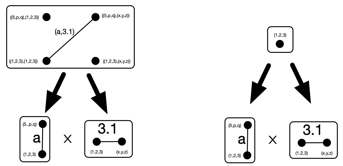
Let’s call the resulting construction the “faux product.” For instance, if X and Y are weighted graphs, then the faux product X\otimes Y has underlying graph the product of the underlying graphs of X and Y, with \mathbb{R} the type of constant weights, and variable weights on every pair of edges from X and Y. These variables coincide if and only if the weights of their two edges coincide.
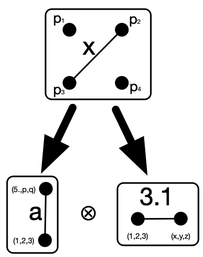
x is not itself a pair of weights, the pair can be recovered via the projection maps which send x\mapsto a and x \mapsto 3.1.We can extend this to limits more generally, such as the following example of stratification which more closely matches our geometric intuitions for how products of graphs ought work.
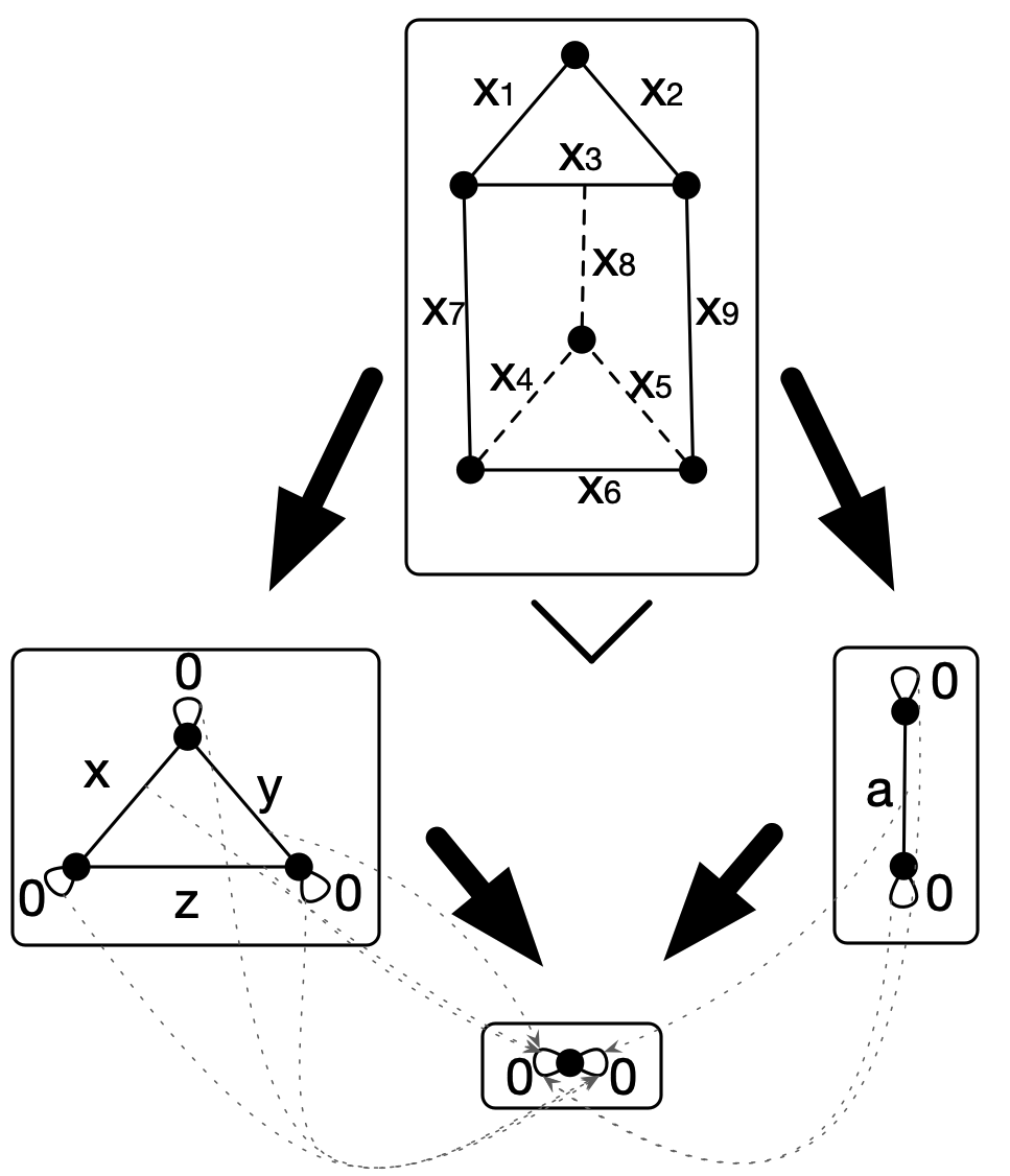
This faux product gets us most of what we wanted. While it’s odd to have turned all the weights into variables, the user can evaluate the weights in the faux product in any way they like after the construction; for instance, by taking the sum or product of the weights from the two factors, or even by the tautological evaluation to a pair in \mathbb{R}^2. Since what evaluation, if any, will be appropriate depends on the application at hand, X\otimes Y is a good place for the general code to leave off.
The abstraction adjunction
It turns out that X\otimes Y has a pretty pleasing categorical description. In general, let i:\mathsf{C}\leftrightarrows \mathsf{D}:R be a coreflective subcategory, that is, i is fully faithful and left adjoint to R. If D has finite products, then there’s always an induced monoidal structure on D given by (A,B)\mapsto iR(A\times B) and with iR(1) as the unit. That is, take the product, and then hit it with the idempotent comonad associated to the coreflective subcategory.3
In our case, the construction above can be modeled by defining the abstraction functor that sends a varacset X on schema S with typing K to the copresheaf \mathrm{abs}(X) on |S| that coincides with X over S_0 and such that, on A\in S_1, we have X'(A)=\sum_{T}\sum_{a:S(T,A)} a(X(T)). That is, over an attribute type, \mathrm{abs}(X) has one combinatorial piece of data for each value of that attribute achieved by some element of X.
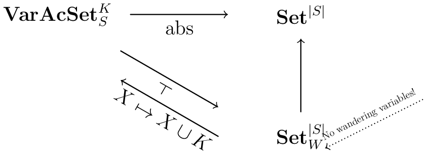
Note that \mathrm{abs}(X) always lacks wandering variables. And in fact, while abstraction is not a right adjoint when valued in \mathsf{Set}^{|S|}, it is a right adjoint when we take the codomain \mathsf{Set}^{|S|}_w to be the full subcategory spanned by those copresheaves with no wandering variables. (Limits in this subcategory take limits in \mathsf{Set}^{|S|} and then throw away wandering variables.) The left adjoint to abstraction simply sends Y to Y\cup K. This is fully faithful (but only because Y lacks wandering variables!) and so we’re in the situation of the previous paragraph.
That is, to summarize, we have an idempotent comonad on the category of varacsets on S with typing K, sending X to the varacset \mathrm{abs}(X) with the same set of constants as X at every attribute type, but with all the attribute values from X replaced with new variables. Then the faux product defined above is precisely (X,Y)\mapsto \overline {\mathrm{abs}(X\times Y)}. 4
Conclusion
Varacsets, originally born out of practical engineering demands for rewriting with attributes, are put on much more stable footing by working out the above theoretical considerations. Just as acsets were not implemented as a slice category, varacsets demonstrate that the right mathematical model doesn’t have to be isomorphic to your implementation: understanding varacsets as a coslice (despite implementing them as a database) is helpful for informing us which operations make sense or do not make sense to perform on varacsets.
Although we focused on rewriting rules in this post, there are lots of other ways to apply attribute variables, e.g. when modeling systems in which some attribute data is unknown. This allows us to \Sigma-migrate data with attributes (via a left Kan extension), as variables give us a universal way to assign attribute values to new data. We’re excited to push varacsets in other directions like this in the future!
References
Footnotes
Note that the length of an edge must equal the Euclidean distance between its source and target to give a semantically valid instance of this schema. This can only be handled perfectly via a Cartesian schema, so we’ll ignore the constraints for now.↩︎
I really just mean to say the forgetful functor is monadic, which is easy to check from the monadicity theorem. But you can explicitly realize such a theory by augmenting S, seen as a theory in the sad logic of a plain category (so only unary operations), with a terminal object and maps from it giving nullary operations for every element of K.↩︎
That this is a monoidal structure follows from the natural isomorphism iR(iR(x)\times y)\to iR(x\times y).↩︎
Limits of other shapes can be constructed in an entirely analogous way: abstract the diagram, take the limit in \mathsf{Set}^{|S|}_w, and then apply the adjoint of abstraction to get your typing functor K back.↩︎