Agent-based modeling via graph rewriting
$$
$$
Note: the code in this post is not kept in sync with the latest developments of AlgebraicRewriting.jl. Please see the official documentation for examples of code that runs with the latest versions of AlgebraicJulia libraries.
Background
Scientists and engineers are often interested in representing the state of the world, S. We might decide to encode this as the set of possible instances of a class,1 or as the set of terms of an algebraic data type,2 or as possible databases on a schema (i.e. \mathsf{C}-sets). We are also often interested in encoding the transition {S \rightarrow S}, a relationship between one state of the world and the next one. If we can communicate this relationship to a computer, then we can execute simulations to see how hypothetical states of the world evolve over time. The question we explore in this post is: what is a good syntax for representing these kinds of functions? Some virtues that we will care about:
- It should be easy for an engineer to construct such functions from simpler ones.
- It should be easy to implement the simulator in a clean, elegant way that does not have complicated edge cases to handle.
- The syntax should be general, such that we can use the same code to perform, e.g., chemistry, robotics, or epidemiology simulations.
- It should be natural to generalize the output of the simulation (e.g. many possible outcomes, S \rightarrow {\rm List}(S), or a probability distribution of outcomes, S \rightarrow {\rm Dist}(S)) without changing much code.
- The structure of the representation should be transparent and introspectable:
- We can write programs to check whether properties of interest hold (e.g. will the program terminate on all inputs?).
- Most importantly, if our representation of the world is fundamentally changed (suppose the world is better modeled by T, rather than S), we can automatically convert our S-simulator to a T-simulator, given some high-level description of the relationship between S and T.
It is difficult to obtain many of these properties when one’s syntax for S is an arbitrary datatype and one’s syntax for the {S \rightarrow S} relationship is just an arbitrary function in your programming language. However, we propose that the syntax of directed wiring diagrams organizing rewrite rules makes these properties more tractable. Although this post will focus on engineering, we can use category theory to describe in more detail what it really means to be a good syntax and show how we can interpret our directed wiring diagrams as agent-based models.
A language for graphical rewriting programs
Example schema
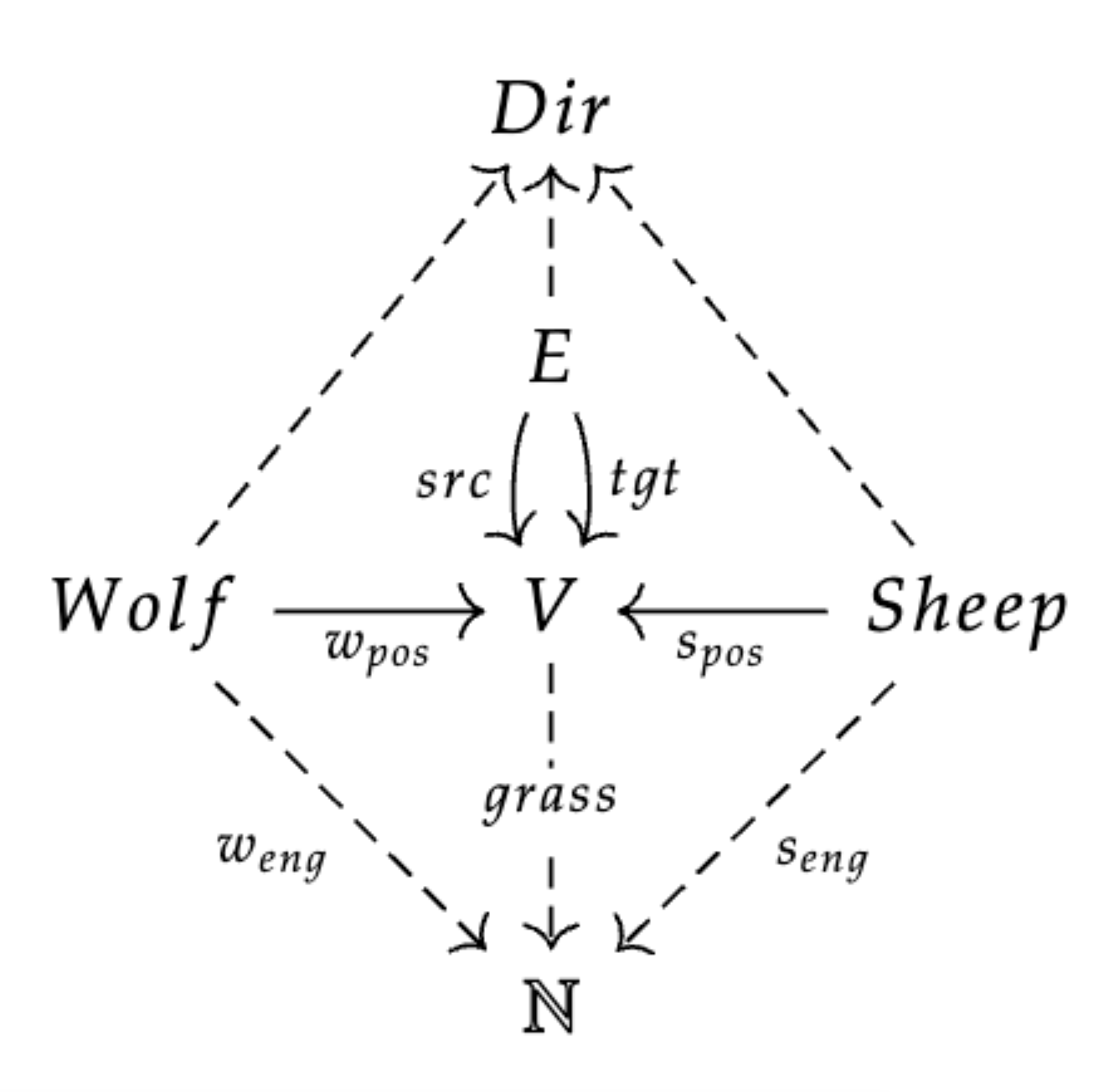
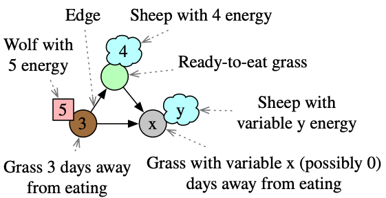
This schema (with objects: Wolf, Sheep, Edge, Vertex, and attribute types: Dir and \mathbb{N}) characterizes states of the world where there are wolves and sheep moving around a directed graph.3 These animals have a position, direction, as well as an energy level. Furthermore, the vertices have grass growing which is also represented by an energy level (let grass=0 mean the grass is ready to eat, while grass=n means there are n days left for the grass to grow). The legend on the right shows how we informally represent instances of this schema, although for simplicity we neglect to visually depict the direction of edges or animals. Using Catlab.jl, we can define this schema:
using Catlab, AlgebraicRewriting
@present SchLV <: SchGraph begin
  (Sheep,Wolf)::Ob
  spos::Hom(Sheep, V); wpos::Hom(Wolf, V)

  (Dir,Eng)::AttrType
  grass::Attr(V, Eng)
  seng::Attr(Sheep, Eng); weng::Attr(Wolf, Eng)
  dir::Attr(E, Dir)
  sdir::Attr(Sheep, Dir); wdir::Attr(Wolf, Dir)
end;

@acset_type LV_Generic(SchLV) # Dir and Eng are abstract
const LV = LV_Generic{Symbol, Int} # Dir is a Symbol, Eng is an Int
const yLV = yoneda_cache(LV) # precompute the 'generic' sheep/wolf/grass etc.
Rewrite rules: primitives for data manipulation
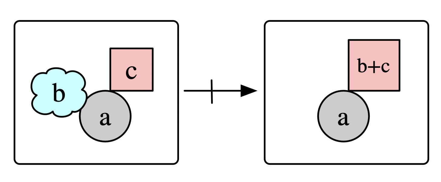
Rewrite rules are good candidates for simple S \rightarrow S building blocks, as they can express interesting dynamics while nevertheless being easier objects to work with than general purpose code.4 This has the data a partial map L\nrightarrow R which says, for any pattern match of L into one’s world of interest, a possible way for the world to update is to replace L with R. For example, the below rule says that, if a wolf and sheep are in the same location, the wolf can eat the sheep and gain its energy units.
Or, in code:
# pattern we're looking for: wolf + sheep on the same V
L = @acset_colim yLV begin s::Sheep; w::Wolf; spos(s)==wpos(w) end
# what we're replacing with: just a wolf
R = @acset_colim yLV begin w::Wolf end
# Get the ID's of the relevant energy variables
L_wolf, L_sheep, R_wolf = [only(x).val for x in [L[:weng], L[:seng], R[:weng]]]
# Combine into a rule: L <- R -> R
wolf_eat = Rule(homomorphism(R,L), id(R);
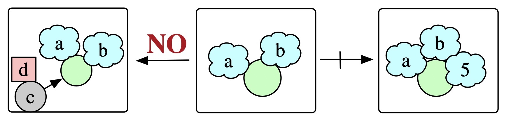
expr=(Eng=Dict(R_wolf => engs -> engs[L_wolf]+engs[L_sheep]),))As another rule, consider two sheep which reproduce if the vertex they share is grassy, unless there is a wolf within striking distance. We can add to the data of a rewrite rule a Negative Application Condition (NAC) which embeds the matched pattern L into a forbidden pattern N with the implied semantics of: the rule cannot be applied to a given pattern L if N also matches.
Or, in code:
# Pattern we're looking for: sheep + sheep on green grass (i.e. grass = 0)
L = @acset_colim yLV begin
  (s1,s2)::Sheep;
  spos(s1) == spos(s2); grass(spos(s1)) == 0
end
# Replacing with: new sheep facing North @ 5 eng
R = @acset_colim yLV begin
  (s1,s2,s3)::Sheep;
  spos(s1) == spos(s2); grass(spos(s1)) == 0
  spos(s2) == spos(s3); seng(s3) == 5; sdir(s3) == :N
end
# Negative application condition
N = @acset_colim yLV begin
  (s1,s2)::Sheep; w::Wolf; e::E
  spos(s1) == spos(s2); grass(spos(s1)) == 0
  src(e) == wpos(w); tgt(e) == spos(s1)
end
NAC = AppCond(homomorphism(L, N; monic=true), false)

# Overall rule
sheep_reprod = Rule(id(L), homomorphism(L,R; monic=true), ac=[NAC])
Rewrite rules are nifty ways of expressing some basic data operations (merging, copying, deleting, adding) and basic logic in a graphical / combinatorial way, i.e. requiring only data rather than general purpose code. But one quickly hits limits in expressivity for what can be accomplished by a single rewrite rule, and there remains the problem of how one structures the execution of many rewrite rules in an organized fashion.
Wiring diagram syntax and control flow boxes
If we view the rewrite rule as system that can be entered and exited in various ways, we might draw it like this:
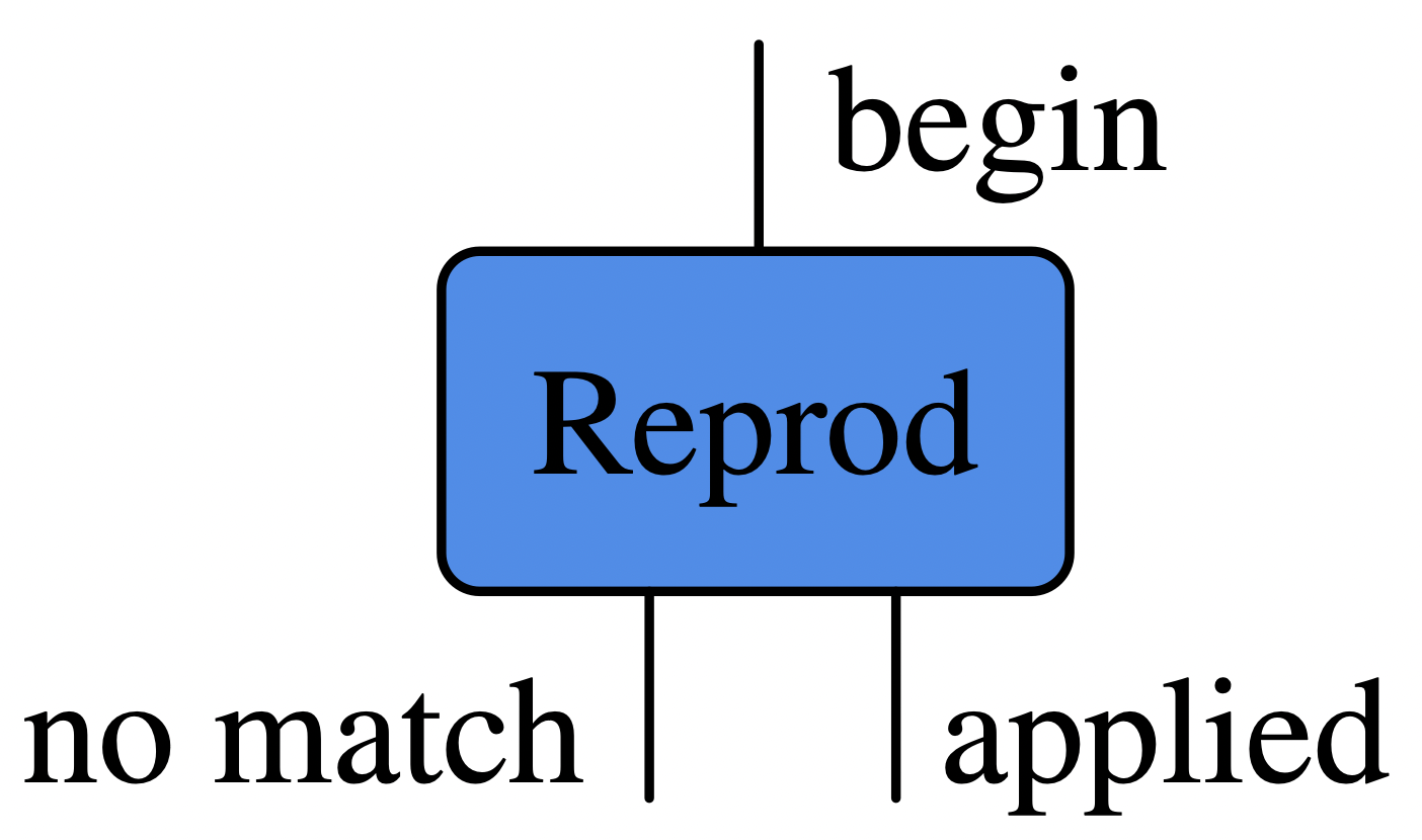
During a simulation, we imagine that the ‘world state’ moves along wires in a diagram like above and is possibly altered by the boxes it passes through. For a deterministic simulation, after entering a box, we will then exit exactly one of the box’s outwires. Although the above box is an example of something that can alter the world state living on the wire, it has no internal state itself. In contrast, we can consider control flow boxes which cannot affect the state of the world yet can have their own state and choose which outwire to exit through as a function of their internal state and the world state.
For example, we can make a repeat3 box which sends the world out the first wire the first three times it run, and subsequently outputs on its second wire. Another box, coin, flips a pseudorandom coin to decide where its output goes. The following diagram communicates a program which first flips a coin, and (if heads) it attempts three times to apply the Reprod rule, ending immediately if at any point it is successfully applied.
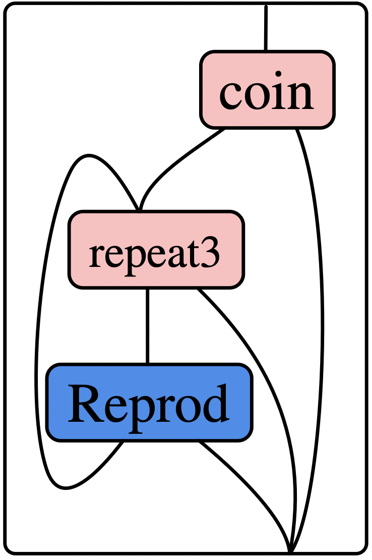
There are many tools at our disposal to construct wiring diagrams like these using Catlab and AlgebraicRewriting. These include calling A⋅B to compose diagrams (which match head-to-tail) in sequence, and calling A⊗B to compose diagrams in parallel. Another powerful tool, which constructs the above diagram in one step, uses the fact that acyclic wiring diagrams can be expressed very naturally using a simple programming-like syntax, where variables correspond to wires, ‘calling a function’ corresponds to feeding wires into a box, and the special syntax [x₁,...,xₙ] corresponds to merging wires together:
mk_sched(
  # 1 *looped* argument
  (r3_loop,),
  # 1 normal argument
  (coin_in,),
  # Bind these names to boxes / wiring diagrams defined elsewhere
  (C = coin, R3 = repeat3, R = sheep_reprod),
  # Construct an acyclic wiring diagram
  quote
    coin_yes, coin_no = C(coin_in)
    R3_input = [r3_loop, coin_yes]
    repeat3_looping, repeat3_finished = R3(R3_input)
    reprod_suc, reprod_fail = R(repeat3_looping)
    output = [reprod_suc, repeat3_finished, coin_no]
    # The 1st argument is fed back into `r3_loop`.
    return (reprod_fail,  output)
end)
Our desired program was not, in fact, acyclic, but by asking for the first n outputs to be looped back into the first n inputs (where n is the length of the first argument to mk_sched), we have a general strategy for making diagrams with loops.
Agent-based modeling
Simulations are often agent-based: instead of thinking of the world state as a monolithic thing S and rewrite rules as functions {S \rightarrow S} that operate on the entire world state, we think of the world state as a collection of agents operating in a shared environment. Updates are relative to a particular agent performing the update.
Thus, we must now consider a state and a particular choice of agent as living on wires, and we must think of rewrite rules as executed “from the perspective of that agent”. Let’s be more precise about what an agent is: given a world state X, we want to pick out a particular substructure of X, meaning our agents are actually maps A\rightarrow X into X, where A describes the shape of the agent. Note that the empty ACSet, denoted as 0, picks out nothing in particular and corresponds to our earlier perspective of a monolithic view of the entire world, X.
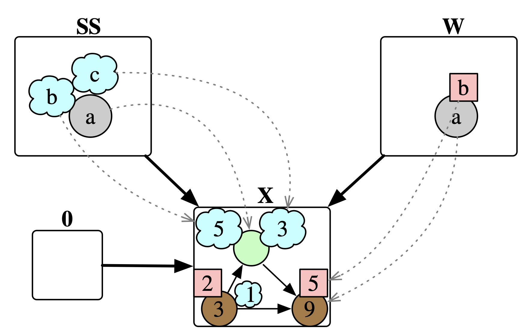
So how does this change our notion of a rewrite rule L \nrightarrow R? We are no longer rewriting a state X but rather a state with an agent: A
\rightarrow X. We need an extra map Agent_{In} \rightarrow L to show, given the agent, how it must relate to our pattern. Furthermore, we need an agent (possibly different) from which to exit the rule application, given by a map Agent_{Out} \rightarrow R. Adding the data W \rightarrow L in the wolf_eat rule transforms the it from “Some wolf eats some sheep” into “This wolf eats some sheep”.
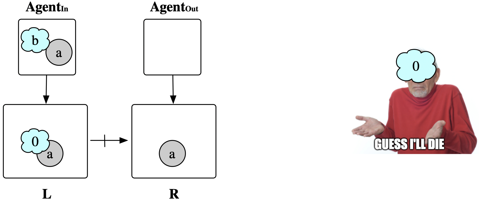
Most often, the incoming and outgoing agents for a rewrite rule are the same. An example where this is not possible is the rule that says “This sheep starves if its energy reaches 0.”
The Query box
The trajectory of the world state while executing a program looks like this:
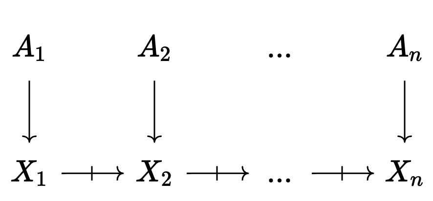
This means it’s possible to take an agent A_i and interpret it in the ‘current’ state of the world, X_n, by composing it with the partial maps between X_i and X_n. This updating of an agent could result in a map which is total (i.e. the agent ‘survived’ the update process) or partial, which would happen if some part of the agent was deleted between step i and step n. We take advantage of this ability to update agents with the last major kind of box, the Query box.
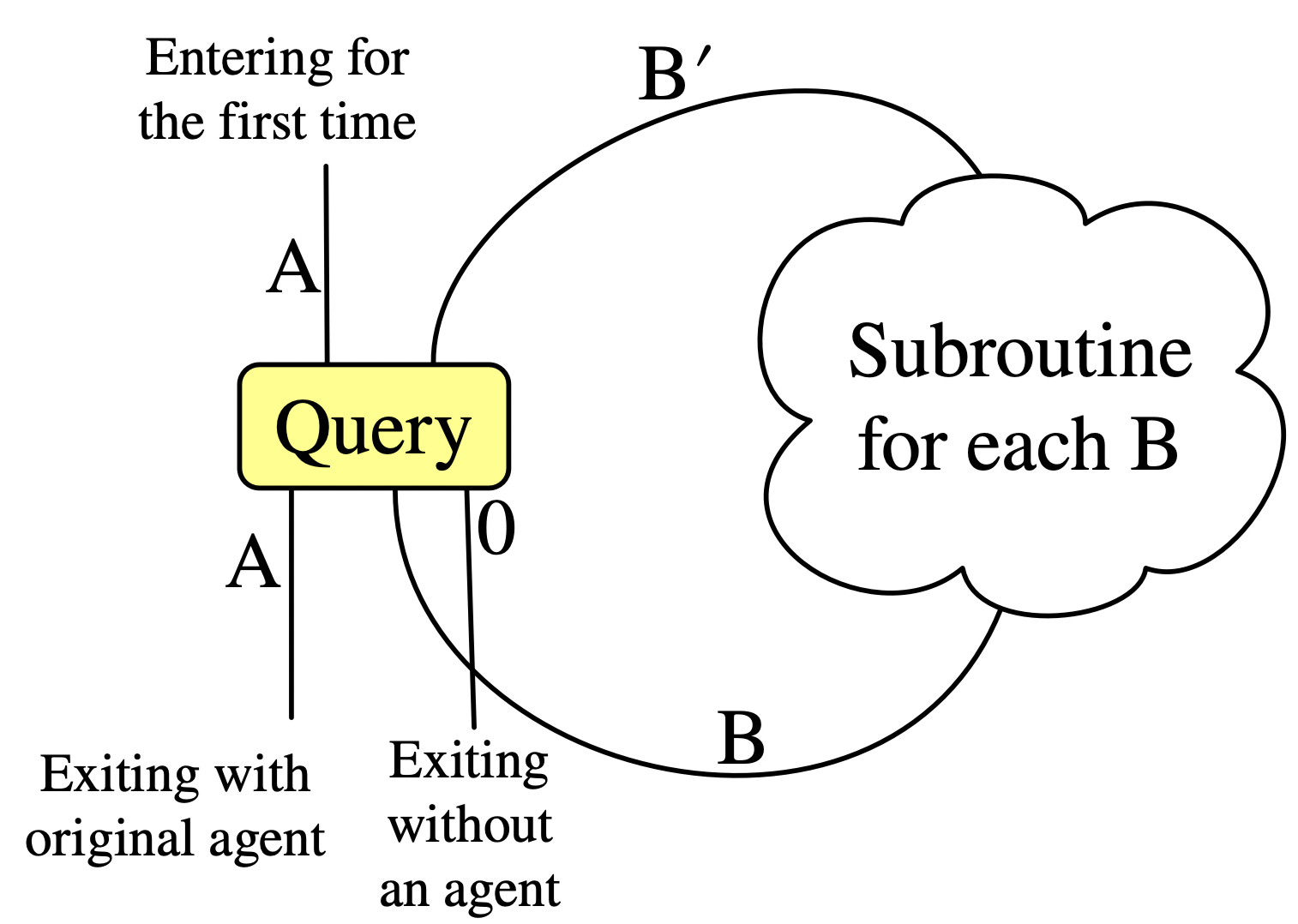
These are yellow boxes which execute a subroutine for each agent of a particular shape. Once this set of matches is found, the query box stores them in its internal state. Each time we return through the second in port, we pop off the next agent in the queue and exit the second out port. Once this queue is empty, we exit out the first port with our original agent. (There is an edge case to consider: what if, while executing the actions of all the sub-agents from the query, our original agent is deleted? In this case we exit a third output door, which has no agent.)
For example, we may wish to organize our wolf-sheep-grass model as a while loop wrapping three for loops, doing some actions per sheep, per wolf, and per vertex.
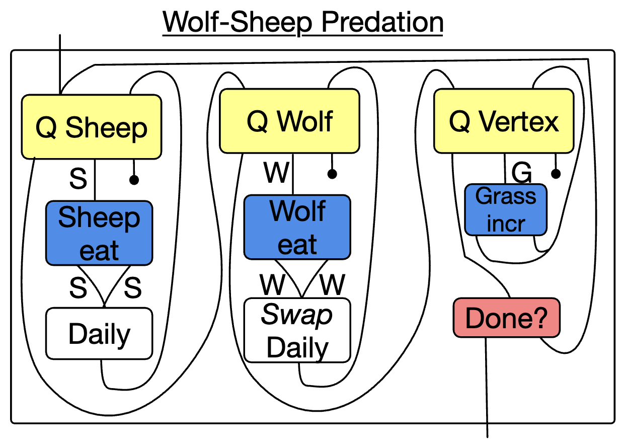
In the figure above, ‘Daily’ refers to another program which performs the actions that are common to both sheep and wolves (e.g. rotating, moving, starving). These are originally defined for just sheep, but by observing the symmetry of wolves and sheep in our schema, we can use a \Delta data migration Swap to automatically translate a Sheep Daily program into a Wolf Daily program.
We may consider other ways of changing our agent type other than the Query box. A simple one is the Weakening box, which is specified by a morphism between agent shapes: B \rightarrow A. It converts A agents into B agents without changing the state of the world. This is because we can precompose this morphism with an agent A \rightarrow X. In particular, for any agent A we can use a weakening 0 \rightarrow A to discard focus on the current agent.
Theoretical underpinning
What it means for a graphical syntax to be formal
Here is a sort of idealized characterization of 2-D drawings of wiring diagrams:
- A wiring diagram can be one of some collection of primitive icons, e.g.:
- perfectly horizontal wires and a
- a pair of crossing wires
- an element from primitive set of boxes with various in ports and out ports
- A wiring diagram can be made by placing simpler ones side by side
- A wiring diagram can be made by placing simpler ones one on top of the other.
The rigid, grid-like diagrams generated by the above rules can be understood as in correspondence to certain expressions in a mathematical theory. Note that the theory comes with its own notion of equality (e.g. id \cdot f = f), and the image has its own notion of equality too: we consider images “up to planar isotopy”, which makes rigorous the notion that it doesn’t matter if you deform the precise locations of things so long as you preserve the same connectivity. Under very special circumstances we can obtain a coherence theorem for a class of wiring diagrams and a particular theory: this says that all equations of the diagrams correspond to equations in the theory (soundness) and all equations of diagrams are a consequence of the theory axioms (completeness). This allows us to relax how rigid our diagrams are depicted while still retaining the formality of terms in a rigorous, mathematical theory.
For example, consider the correspondence of wiring diagrams (without feedback loops) to a theory of symmetric monoidal categories (SMCs) with monoidal unit I and a supply of monoids.
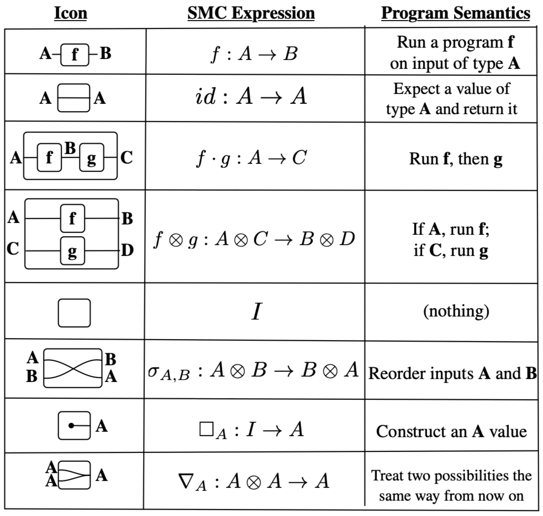
Once we have interpreted our wiring diagram as a morphism in a certain kind of category, applied category theory seeks to interpret the morphism in some real world context, provided that real context can be given the structure of a category (including the satisfaction of required axioms). For a certain toy model of programs with control flow, the third column describes how one can interpret the mathematical expressions in the setting of programs, such that compositions of diagrams can rigorously be interpreted as compositions of programs.
To show the correspondence of the first two columns in action, consider the below composite wiring diagram, which takes for granted a morphism f: A \otimes B \rightarrow A \otimes B \otimes C. Dotted lines are added to visually guide you in parsing the various icons, which are composed vertically and horizontally.
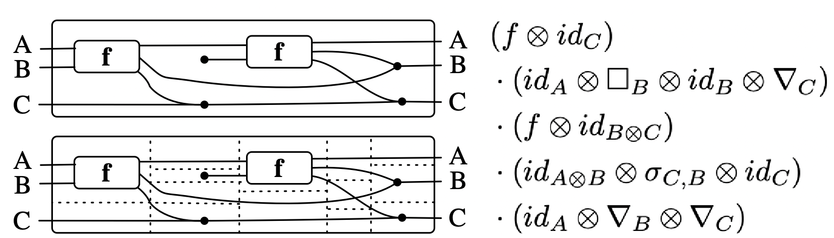
Thanks to a coherence theorem, we can rest easy knowing that the diagram has an unambiguous formal meaning, even if some of the lines are a bit wiggly and don’t exactly match one of our icons.
Some great follow-up reading for what it means for these diagrams to be formal are Baez and Stay (2011) and Selinger (2011). Also, a great application of graphical languages is pedagogically described in Pawel Sobocinski’s blog Graphical Linear Algebra.
What’s in the box?
To connect the above ideas to the graphical language explored in the bulk of this post: the syntax of directed wiring diagrams (with feedback loops) can be given the semantics of a traced SMC, though unpacking what that means theoretically is beyond the scope of this post. In a programming-like setting (the final column in the table above), this corresponds to while-loop style iteration.
In Brown and Spivak (2023), a theoretical underpinning of this work is proposed. The primary contributions are formulating a general theory of discrete dynamical systems, making progress towards showing that the relevant category is traced monoidal, and then showing how this informs the implementation of the graph rewriting programs described in this post. This involves enriched category theory, the language of polynomial functors, and is parameterized by a polynomial monad, such as:
\text{Maybe}=\mathcal{y}+1,\qquad \text{List}= \sum_{N:\mathbb{N}}\mathcal{y}^N, \qquad \text{Dist}=\sum_{N:\mathbb{N}}\Delta_N\mathcal{y}^N
where {\Delta_N=\{P:N \to [0,1]\ |\ 1=\sum P(i)\}}. It is beyond the scope of this post to rigorously explicate this formalism, which is gently introduced in Niu and Spivak (n.d.). However, to provide some intuition for how, in practical ways, this formalism informed the design of the software infrastructure that represents and executes these graphical programs: consider a box swap-x2 which has two inputs. Initially, it behaves by swapping the inputs, but once the left inport has been entered twice it behaves like a pair of parallel wires.
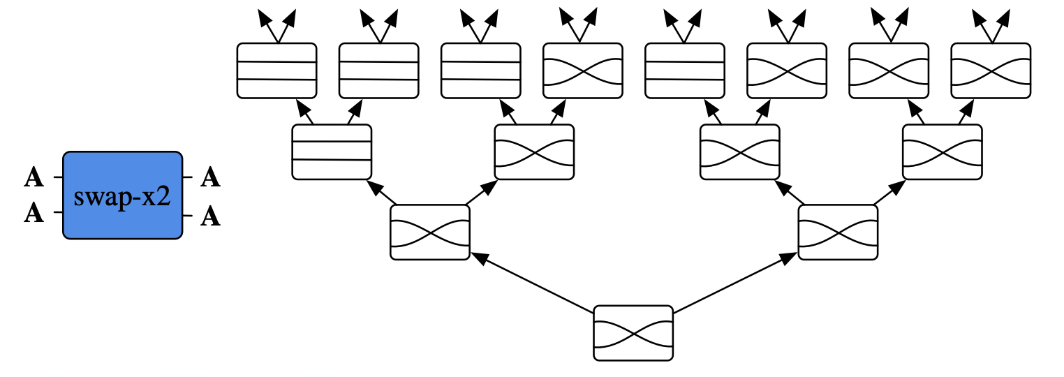
The math dictates that what actually should go into this box is a “behavior tree”, where the branching of the tree is dictated by the number of input wires. For every input, we specify how the behavior changes by pointing to a new behavior tree, whose nodes indicate how the input is transformed into outputs.
All of the rewriting primitives (e.g. Rewrite, ControlFlow, Query, Weaken) are implemented in this generic manner, meaning just one implementation (i.e. behavior trees) needs to be written, rather than many special cases for language primitives. Furthermore, the language can be extended, with the formalism allowing us to not worry about unforeseen consequences that follow from ad hoc extension of the language - we have a precise specification for what structure a new primitive needs to satisfy.
The setting of polynomial functors is so expressive that the interfaces of boxes, their internals, their infinite behaviors, and monadic effects on their outputs (like \text{List} and \text{Dist}) are all encompassed in the same formalism, which leads to a cleaner and more general implementation than what would have been arrived upon if the problem were approached head-on in a traditional engineering style.
Conclusion
The virtues of this approach largely come from the fact that neither code nor arbitrary functions are in principle required to specify our dynamical system S \rightarrow S. Rather than arbitrary functions (which are hard to manipulate and reason about) being the input, we automatically generate our simulator program from static, graph-like data. While we happen do this in Julia, this could in principle be done in any language because our understanding of a graph rewriting program is mathematical, rather than dependent on implementation details. In collaborations involving multiple teams, it can be helpful that the data of these programs can be serialized in a language-agnostic way.
I have also personally found it immensely useful to be able to apply functorial data migration (see Spivak (2012)), e.g. swapping sheep and wolves, to allow high level reuse of programs in different contexts, which can be done cleanly and rigorously when one’s model is expressed via combinatorial data rather than low-level code.
Although there was not space to describe how all of the virtues listed in the introduction are facilitated by this formalism, I hope you’re intrigued by the possibility of structuring your model of the world’s dynamics in this formalism. Furthermore, I hope this case study in applied category theory encourages you to look into other kinds of scientific or engineering tasks can be made more scalable and maintainable through these kinds of abstractions.5
References
Footnotes
E.g., if we live in an object-oriented paradigm:
↩︎class WorldModel { int NumIDs() const; // id's for objects in the world int LoadRobot(const string& fn); int AddRobot(const string& name,Robot* robot=NULL); void DeleteRobot(const string& name); int main(int argc,const char** argv) { WorldModel world; //create a world double dt = 0.1; //between printouts while(sim.time < 5) { //run the simulation sim.Advance(dt); //move the sim fwd sim.UpdateModel(); //update the world cout<<sim.time<<'\t'<<world.robots[0]->q<<endl; } return 0; } }E.g., if we live in a functional paradigm:
↩︎data Particle = Particle { idx :: Index, pos :: Position, vel :: Velocity} type Model = [Particle] simulate :: Display -- Window config -> model -- Model -> (model -> Picture) -- Draw function -> (Float -> model -> model) -- Update function -> IO ()This is inspired by Netlogo’s wolf-sheep predation model. A more faithful reproduction of that model’s dynamics is found in the docs of AlgebraicRewriting.jl; in this post, we’ll focus on showcasing a more diverse set of AlgebraicRewriting’s features.↩︎
For more background and computational details, see Brown et al. (2023). See also Angeline’s description on this blog.↩︎
This work came about through conversations very much akin to the example conversations between the domain expert (me) and ACT expert (David Spivak) in David’s What Are We Tracking talk, so I encourage you to watch that to get inspiration for other potential fruitful collaborations with mathematicians.↩︎